Reference
The sections below summarize the actions associated with each menu item. The links will take you to the relevant section of the Notes.
File menu
New: Clears output window.
Save output: Saves contents of output window to text file.
Load data: Loads an Mstat data file (which has an ".ijd" extension) into the current session. If you have already defined variables, you will be given a chance to save the current definitions to a file. If the file to be loaded contains variable names that are already in use, the current definitions will be replaced in memory by the new data. The format for storing variables used by Version 3.0 and later differs from that used by previous versions, which used the ".jd" file extension. However, you can load data files generated by earlier versions and the data will be interpreted correctly.
Save data: Saves the variables in the current session to a data file. Mstat data files are text files that are J scripts beginning with the line "NB. ijd file". You can edit the file with any text editor, but probably shouldn't unless you are familiar with the J programming language. The keyboard shortcut Ctrl-s applies this function.
Import data: You can import data into an Mstat session from a tab-delimited or comma-delimited text file, such as those produced by spreadsheet programs like Microsoft Excel or LibreOffice Calc. Version 6.2 and later have improved the responsiveness of the import function for very large data tables and added the ability to import compressed (gzipped, extension .gz) files. See the example above in the tutorial.
Export data: Regular and indicator variables can be saved to a comma-delimited (csv) text file, which can be opened in your favorite spreadsheet program.
Export tables: Save selected tables as CSV files to the chosen folder.
Printer setup: Choose the default printer, margins, and orientation. This dialog is also accessible from the Preferences dialog (see below).
Print: Prints contents of output window to default printer. The keyboard shortcut for this function is Ctrl-p.
Preferences: Sets program preferences through the following dialog box
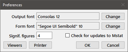
The Preferences item is in the Mstat menu on macOS.
Press the appropriate Change button to call up a font dialog box to choose a font for the output window and the printer, or all of the program dialog boxes (Form font). You should select a monospaced font for the output window and printer so that tabular material lines up correctly. The "Consolas" font included in recent versions of Windows works well, as do Andale Mono, Monaco, and Ubuntu Mono. All of these fonts provide clear distinctions between 0 and O, 1 and l, and are often touted as "Programmer fonts" (just search the web). The form font is a matter of taste, but choose a size that does not result in truncation of the labels on the dialog boxes. The Signif. figures edit box determines the number of significant figures displayed in the output and must be between 2 and 9. Changes made through the Preferences dialog are immediately written to disk in the file "mstat7.ini" within the .mstat7 directory in your home folder and will apply for the remainder of the current session and for subsequent sessions. Beginning with version 5.3, minor updates to Mstat can now be downloaded and installed automatically. To enable automatic (weekly) checking for an updated version of Mstat, select the checkbox in the dialog.
Pressing the Viewers button will bring up the following dialog:
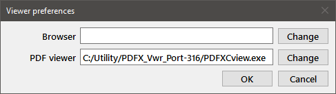
The Browser is used for visiting the Mstat website (from the About dialog) and for displaying the Help file. The PDF viewer is used for optimal printing of plots. Generally, the system default applications for these functions will be used by Mstat (the edit box will be empty in that case). However, you can specify alternative applications using this dialog. For example, if you have Adobe Acrobat installed on your system, you may prefer to use Preview on macOS or a program like Foxit Reader on Windows because they load more quickly. Press the appropriate Change button and choose the desired application from the file open dialog. Press OK to save the changes. To revert to the system default applications, clear the entries in the two edit windows and press OK.
Pressing the Printer button will bring up the Printer preferences dialog:
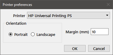
Choose the desired printer from the dropdown list at the top of the dialog. You can also specify the orientation for the output using the Portrait or Landscape radiobuttons, and the margin (in mm) from the edit box. Pressing OK saves these choices, which are persistent between Mstat sessions.
Exit: Exits the program. If you have not already saved the data or output, you will be prompted to do so before exiting. The keyboard shortcut Ctrl-q will also exit the program. Note that this item is on the Mstat menu in macOS.
Edit menu
Annotate: Choosing annotate allows you to enter or edit text in the output window, so that you can make notes regarding your analyses that will be saved or printed with the rest of the output.
Undo: Available only when in annotate mode, causes the contents of the output window to revert to what it was before entering that mode.
Wrap: This menu choice will toggle wrapping of the text in the main window.
Scratchpad: The Scratchpad allows you to perform calculations in J notation. Enter a valid J expression in the edit box, press the return key, and the results of that expression will appear in the edit window, as shown below. Press the Reset button to clear the edit window, the Help button to print a short help message to the window, or the Done button to dismiss the Scratchpad. A brief summary of J notation is included in the Appendix. Temporary variables may be defined in the Scratchpad and are available until the Mstat session is terminated. For example, to assign the vector 1 2 3 4 5 to the variable a, enter
a=: 1 2 3 4 5
in the edit window.
The Scratchpad is meant to provide a safe environment for doing on-the-fly calculations.

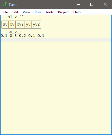
Terminal: Opens a fully functional J terminal window. Enter any valid J expression and press return to see the result. You can also press the Terminal button in the toolbar. In contrast to the Scratchpad, there are no real limitations on what you can do, so be careful. Note that pressing the close button (upper right corner) of the Terminal window will end the Mstat program. You should use the Terminal menu choice or toolbar button to close the Terminal window.
Data menu
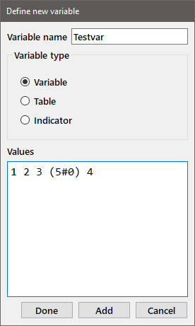
New: Adds a new variable to the session; you may also use the shortcut Ctrl-n. See the tutorial for a discussion of this dialog window. For regular variables, the data in the edit box is evaluated as follows. The program first attempts to evaluate the contents as a list of simple numbers (e.g., 2 3 -5 1e-5 assigns a list of four numbers to the variable). If that attempt fails, the portions that are not simple numbers are evaluated as J expressions. It is a good idea to enclose the J expressions in parentheses. In the dialog box below, the variable "Testvar" is assigned the list of values [1 2 3 0 0 0 0 0 4].
Tables or Indicator variables may be entered by choosing the appropriate radiobutton. When entering a table, the edit window is set such that the lines do not wrap at the edge of the window so that complete lines can be entered. You can change the size of the dialog so that the all of the lines of the table are visible in their entirety. The contents of the edit window do wrap at the edge of the window for variables and indicators. Entering indicator variables presents an additional issue since some of the values may include spaces. If you are entering data from the keyboard, you can enclose an item that contains spaces in double quotes to insure that the item is properly saved. Alternatively, the items in the edit window can be delimited by tabs (e.g., when a row from a spreadsheet is copied) or line feeds (e.g., when a spreadsheet column is copied to the window). If tab or line feed characters are present in the edit window, those characters are used to parse the contents of the window. In that case, both spaces and quote symbols are preserved in the items.
Edit: Allows you to edit the contents of a variable. The shortcut Ctrl-e will also open this dialog. Use of J notation is allowed in the edit window, as described for the Data>New entry. See the example in the tutorial. The discussion above in New regarding table and indicator variables applies here as well.
Show: Prints the contents of one or more variables to the output window.
Classify: Uses an indicator variable to generate new variables consisting of a subset of the data contained in a variable. The indicator and variable must have the same number of values in the appropriate order. See the discussion in the tutorial.
Convert: The choice Ordered table to variables converts a table variable in which the columns follow a natural order into simple variables on a row by row basis, converting each observation in the row to a numerical value equivalent to the column number. The names of the variables are constructed as "TableName_RowName". For example, the table "hyperplasia" contains data from histological analysis of sections from animals homozygous for one of several alleles at a particular locus. Each section is evaluated and the level of hyperplasia in the tissue is graded as absent, moderate, or severe. After selecting the Data > Convert >Ordered table to variable menu choice, the "hyperplasia" table is chosen from the dialog box. The data in the table are displayed in the form below:

Note that the window may be resized to show the whole table. Choose the appropriate radiobutton, depending on whether the columns are in increasing or decreasing order. In our example, the observations in the first column will be assigned a value of 0, those in the second a value of 1, and those in the last a value of 2. Showing the resulting variables gives the following output.
hyperplasia_wt
0 0 0 0 0 0 0 0 0 0 1 1 1 1 2 2 2 2

hyperplasia_m1
0 0 0 0 0 1 1 1 1 1 1 1 1 2 2

hyperplasia_m2
0 0 0 0 0 0 1 1 2

hyperplasia_m3
0 0 0 1 1 1 1 1 1 1 2 2 2 2 2 2 2 2
Choosing Data > Convert > Table to variables allows you to select a table and convert the rows or columns to variables using the same approach as was used to import variables from a CSV file (see the example in the tutorial).
You can also convert a regular variable into an indicator variable or an indicator into a regular variable. The latter only makes sense if the indicator variable contains 'numeric' data.
Transform: Creates a new variable that is a transformation of an existing variable through the following dialog box:
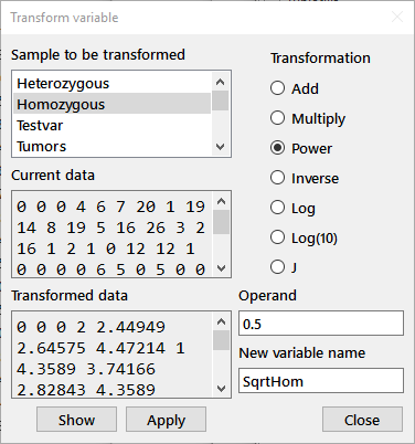
Highlight the variable to be transformed in the listbox at the upper left ("Homozygous" in this case) and choose the radiobutton for the appropriate transformation. Enter an operand for the transformation and a name for the new variable in the indicated edit boxes. In the example above, a new variable "SqrtHom" is being defined as the square root (0.5 power) of the variable "Homozygous". Pressing the Show button will display the results of the transformation; the Apply button will enter the new variable into the current session. Note that you can easily make a copy of a variable under a new name by Adding 0 or Multiplying by 1. The J transformation allows you to enter any allowable J expression as the Operand to perform a functional transformation. For example, the expression
^.@(1&+)
will transform the data by adding the value 1 to it and taking the natural log. The on-screen, dialog help (see below) contains other useful J phrases.
Rescale: A convenience function that will transform multiple variables by dividing by a constant. Doing so may be useful when plotting data. For example, you want to rescale the following data to "millions".
Tot_Federal
5.927e8 6.219e8 6.099e8 6.505e8 6.003e8

Tot_Nonfed
1.69e8  1.519e8 1.738e8 1.685e8 1.77e8
Choosing Rescale from the Data menu gives the dialog box:
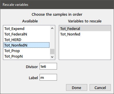
Selecting the relevant variables, and entering the indicated values in the Divisor and Label edit boxes gives you two new variables:
Tot_Federal_m
592.7 621.9 609.9 650.5 600.3

Tot_Nonfed_m
169   151.9 173.8 168.5 177
Delete: Select the variable type using the radiobuttons. Choose variables from the Available listbox by double-clicking or highlighting them and using the Add button. Pressing Done will delete the selected variables from memory.
Clear: Remove all variables from the current session (I hope you saved them first).
Analysis menu
Descriptive: Descriptive statistics will be printed to the output window for the set of variables chosen in the dialog box. See the tutorial.
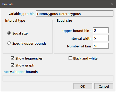
Bin data: Prints (and optionally plots) the sample distribution for one or more variables. Choose the desired variables from the multisample dialog and the Bin data dialog (below) will be displayed. The selected variables are listed in the edit box at the top of the dialog. Choose the interval type from the radiobuttons at left. If Specify upper bounds is chosen, enter the upper bound for each interval in the edit box at the bottom of the dialog. Parameters for equal size bins are entered as indicated in the group of three edit boxes. After specifying the upper bound of bin 1 and the interval width, press the Enter key (while the cursor is in the interval width or number of bins edit boxes); the program will suggest a number of bins such that the largest observation is placed in the second last bin. Intervals are right-closed, i.e., each bin includes observations less than or equal to the upper bound for the interval and greater than the previous upper bound.
Check Show graph to display histograms for the binned variables. The Black and white option sets the plot colors to shades of gray as a starting point; all color options are available from the Plot parameters dialog. The number of observations in each bin is printed to the output window, along with the frequencies if Show frequencies is checked.
Kaplan-Meier analysis: The Kaplan-Meier (product limit) method may be used to estimate survival distributions when some of the samples are censored. For each group, the failure (or other event) times and censoring times are stored in independent variables. Choose the appropriate failure and censoring times for each group using the Paired-sample dialog box as shown below. The available variables are shown in the Event times and Censor times listboxes. The value "(None)" is also included at the top of the each list. For each group, select the appropriate variable for the event times on the left and censoring times on the right (choose (None) if no samples were censored in that group), then press the Add button. The chosen pairs of variables are displayed in the box labeled Event, Censor pairs.
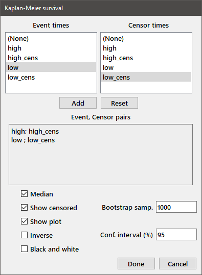
If you want to estimate the median survival by the bootstrap method, select the Median checkbox and enter the number of bootstrap samples desired and the size of the confidence interval in the edit boxes at the right of the dialog. To display the survival curves, select the Show plot checkbox. If the Show censored checkbox is selected, censoring times will be displayed on the plot as tic marks on the survival curves. The Inverse checkbox will show a plot of "Cumulative Death Rate" rather than "Survival". When all of your choices have been made, press the Done button.
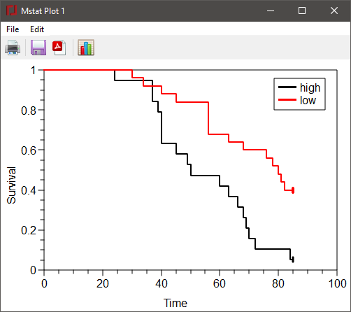
A portion of the results for the above dialog and the survival plot are shown below.
Kaplan-Meier survival
Events: high
Censored: high_cens
Time   Events   At risk    Survival
24     1        19        0.9474
37     2        18        0.8421
39     1        16        0.7895
40     3        15        0.6316
45     1        12        0.5789
…
69     1        5         0.2105
70     1        4         0.1579
72     1        3         0.1053
84     1        2         0.05263
Median survival (95% CI; 1000 samples): 50 (40,68)
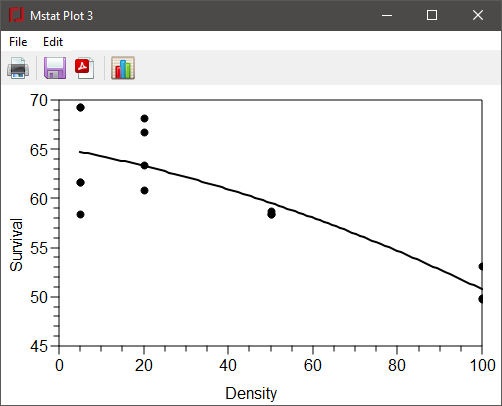
Regression: Straight line, polynomial, or multiple linear regression can be chosen from the following dialog box.

The Y variable is chosen from the drop box, and the X variable(s) are chosen from among Available variables by double-clicking (or drag and drop). More than one X variable can be chosen only for the Multiple regression type. Checking Constant includes a constant term in the regression and checking Plot will display a plot for Line or Polynomial regression. The dialog box above generated the following output:
Polynomial regression, order 2
Y: SurvEggs  X: DensEggs
y = c0 + c1*X + c2*X^2

c    Parameter    std. dev.
c0        65.16      3.175
c1     -0.08048     0.1891
c2   -0.0006356   0.001756

     s2           37.16
     R2           0.7269
     N            15
The regression equation is printed, followed by a table with the value of each parameter and its standard deviation. R2 is the correlation coefficient for the regression and N the number of data points.
The plot generated by this regression is shown below, following the use of Modify plot to change the X and Y axis labels, the X range and the marker size. Note that line styles for these plots are limited to solid or dotted.
Binomial conf. interval: Computes a confidence interval for binomial data. In the dialog box, enter "x N" where x is the number of successes and N the number of trials. The dialog below generated the following output (the upper and lower confidence limits are in parentheses):
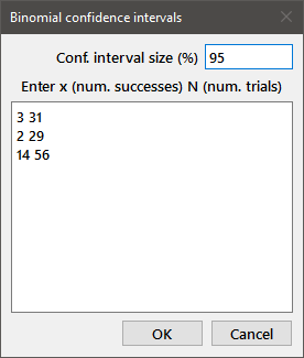
Binomial 95% confidence interval
x = 3, N = 31
p = 0.09677 (0.02042, 0.2575)

Binomial 95% confidence interval
x = 2, N = 29
p = 0.06897 (0.008464, 0.2277)

Binomial 95% confidence interval
x = 14, N = 56
p = 0.25 (0.1439, 0.3837)
Bootstrap confidence interval: Estimates a confidence interval for the mean, median, or variance of a variable using the bootstrap method. In the dialog box, choose one or more variables and enter the confidence interval size and number of bootstrap samples in the appropriate edit boxes. Choose the desired estimators (mean, median, variance) by selecting the appropriate checkboxes. A sample dialog box and the resulting output are shown below. The upper and lower confidence limits are shown in parentheses.
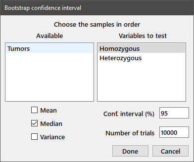
Bootstrap 95% confidence interval, 10000 trials
Sample: Homozygous
Median  2 (1, 5)

Bootstrap 95% confidence interval, 10000 trials
Sample: Heterozygous
Median  11 (5, 18.5)
Ratio: Computes the mean and standard deviation for one or more variables when taken as a ratio with another variable. This procedure is useful for reporting normalized values (i.e., a value as a fraction of some control). The variable corresponding to the denominator is chosen in the lower list box. One or more variables for the numerators are chosen from among Available variables. The output generated is shown below the dialog box.
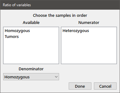
Ratio of variables
Denominator is Homozygous
Numerator    Mean   Std. dev.
Heterozygous 3.472  5.811
Plot menu
Mstat can be used to generate several types of plots in addition to those described above for the Analysis menu (Bin data, Regression, Kaplan-Meier). For a description of the menu choices within the plot window, see the section Plot window menus toward the end of the Reference section. A representative sample of the various plot types is shown below.

|

|

|

|

| |
Load plot: Use this menu choice to re-open a previously saved Mstat plot. You can then make further changes to the appearance of the plot, or save it as a PDF or EPS file. One important thing to note is that Mstat plots are not "live"; the data used to generate the plot are saved in the plot file and subsequent changes to the variables that were used for the plot are not reflected in the plot window.
Dot plot: For a description of the menu choice Dot plot, see the tutorial.
Bar graphs: Five types of bar graphs are available from the Plot > Bar graphs menu choice: Grouped, Grouped with SD, Stacked, Floating, and Area. For bar graphs that include standard deviations choose the variables in the desired order from the paired sample dialog box. For the other plots, choose variables in the multisample dialog box, as shown below. For Grouped, Stacked, and Area graphs, the variables are displayed in the plot left-to-right or bottom-to-top. For a Floating bar graph, the first entry represents the bottom of the floating bar. You can also reorder the bars in ascending or descending order by checking the Order bars checkbox and choosing the appropriate radiobutton. For the grouped bar chart, the ordering is determined by the magnitudes of the values in the first selected variable. For the stacked, floating, and area charts, the order is determined by the sum across all of the variables.
The X-axis labels may be chosen from among the Indicator variables listed in the dropdown box at the lower left. Note that these entries may have spaces, as long as the items were delimited by quotes when the variable was defined. Each data and label variable must have the same number of values. The Black and white checkbox sets the initial plot colors to shades of gray.
The data from the dialog below were used to generate the top-left plot on the previous page.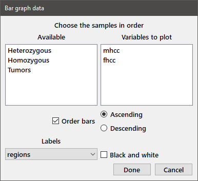
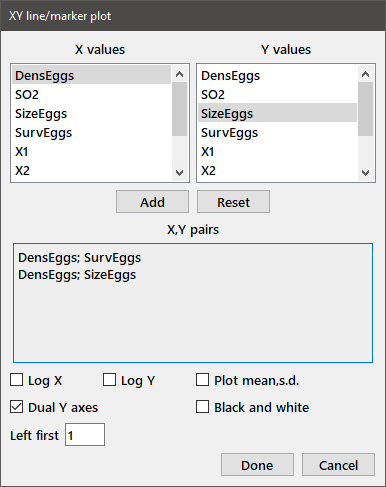
XY plots: The first three choices for this sub-menu, Markers, Lines, Both marker/line, can be used to generate X-Y scatter plots. For each data set, choose the X and Y values from the Paired-sample dialog, as shown below. Either the X or Y axis (or both) can be displayed on a log scale by selecting the appropriate check box. This choice is ignored if one or more of the data points has a value less than or equal to zero. Regardless of which plot type is chosen, the plot can later be modified to include markers, lines, or both. When multiple samples have the same X value, the line is drawn through the mean of the Y values. Selecting the Plot mean,s.d. checkbox will plot the mean and standard deviation for each group of X values, rather than the individual observations.
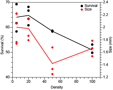
Data with distinct ranges can be plotted using different left and right y axes. Choose all of the XY pairs for the left axis first, and then choose those for the right axis. Check the Dual y axes box and enter the number of variables using the left axis in the Left first edit box. An example dialog and plot with one variable plotted for each y axis is shown below.
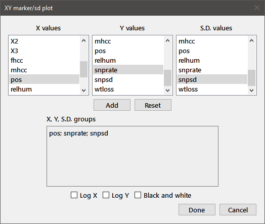
Select the Marker with SD choice from the XY plots sub-menu to plot XY data with their associated standard deviations when you have already computed the means and standard deviations. For each data set, choose the variables containing the X, Y, and SD values from the Triplet sample dialog as shown below.
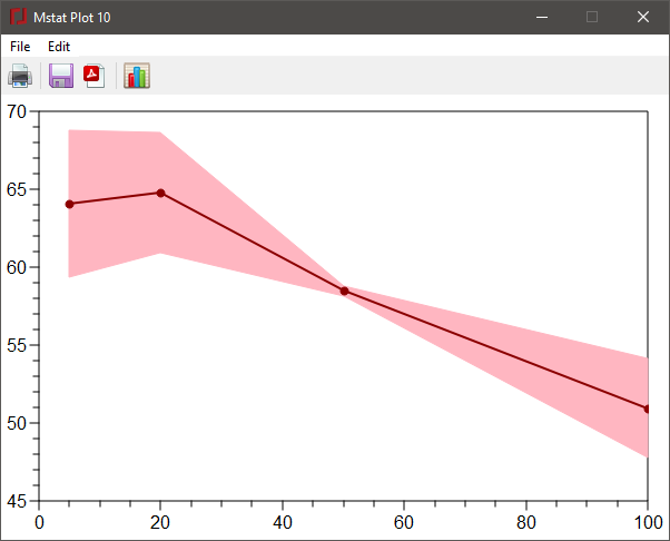
The final XY plot type is the band plot. For variables with multiple Y values for each of a series of X values, you can choose to plot the median at each x-value surrounded by a band representing the range from the first to third quartile. Alternatively, you can plot the mean y-value with the band representing the indicated confidence interval. Choose the XY pairs as for the other plots and then select the Quartile or CI radiobutton as appropriate. In the latter case, enter the desired % CI in the edit box. The band will be shown in a lighter shade of the color for the marker/line.

Test menu
For a complete description of each statistical test, follow the hyperlink to the corresponding section of the Notes. Choosing a test will call up a Two-sample, Multi-sample, or Paired-sample dialog box as appropriate. An example of the Two-sample dialog is given in the tutorial for the Wilcoxon rank sum test—select one sample in each of the two list boxes and choose the one- or two-sided radiobutton. The Multi-sample dialog box is similar to that shown for Descriptive statistics in the tutorial, except that it may contain one- and two-sided radiobuttons (or other controls) if appropriate. Select the samples in order by double-clicking in the Available variables list box. The selected sample will be moved over to the Variables to test list box. You can also move variables between the list boxes by dragging and dropping. The Paired-sample dialog is shown above in the description of the Kaplan-Meier analysis.
Wilcoxon: Performs the Wilcoxon rank sum test using the variables selected in a Two-sample dialog. See the tutorial for a discussion of the method used to compute P-values for the rank sum test.
Signed rank: Performs the Wilcoxon signed rank test using the variables selected in a Two-sample dialog. The variables, e.g., "Before" and "After", must have the same number of values and should represent paired observations in the same order.
Kruskal-Wallis: Performs the Kruskal-Wallis test using two or more variables selected in a Multi-sample dialog.
Jonckheere: Performs the Jonckheere-Terpstra test against an ordered alternative (e.g., dose response) using two or more variables chosen (in order) from a Multi-sample dialog.
Miller jackknife: Tests for differences in variance between two groups selected with the Two-sample dialog using Miller's jackknife method. One- or two-sided tests may be performed.
Conover: Tests for differences in dispersion among two or more groups selected with the Multi-sample dialog using Conover's method. Squared-ranks are computed for the magnitudes of the differences between individual values and the median for each group.
Goodness of fit: Performs the Chi-square goodness of fit test for a 1 × c table. Variables containing the Observed and Expected values are chosen from the two list boxes, as indicated in the Two-sample dialog below. The number of values in the two variables must be identical. The Expected variable may either be Expected Values (sums to the same total as the Observed) or Expected Frequencies (sums to 1.0), with the appropriate type chosen from the radiobuttons below. The number of estimated parameters must be entered in the edit box. For example, consider the following data:
Genotypes
1 9 9

GenotypeFreq
0.25 0.5 0.25
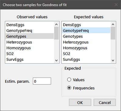
The dialog above gave the following results.
Chi-square goodness of fit test

Genotypes (Observed)      1      9     9
GenotypeFreq (Expected)   4.75   9.5   4.75
X2 = 6.789 P = 0.03355 (2 degrees of freedom)
Note that the expected numbers rather than the frequencies are displayed in the "GenotypeFreq (Expected)" line.
Fisher exact: Fisher's exact test is performed for one or more 2 × 2 tables chosen from a Multi-sample dialog.
Barnard exact: Barnard's exact test is performed for one or more 2 × 2 tables chosen from the dialog below.

Tables are selected as from the multi-sample dialog box. All tables must have either fixed row or column totals, which is indicated by selecting the appropriate radio button. For tables with the largest fixed total (row or column) equal to 25 or less, Barnard's CSM method is used to determine the critical region for the test (CSM-order). If either of the fixed totals exceeds 25, the critical region consists of those tables with a Fisher's exact P-value that does not exceed that for the observed table (F-order).
Barnard's exact test (CSM-order)
Table StrainVar
Fixed rows
          Tumor   Tumor-free   Total
Strain1   1        20          21
Strain2   5        12          17
Total     6        32          38
P(two-sided) = 0.04886
Chi-square: The Chi-Square test is performed for one or more r × c tables chosen from a Multi-sample dialog.
Partition table: One or more r × c tables may be selected from the Multi-sample dialog box. Each table is partitioned into (r-1)(c-1) tests with 1 degree of freedom. Radiobuttons allow you to choose whether a Chi-square test or likelihood ratio test is performed.
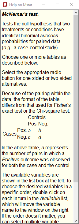
McNemar: For one or more 2 × 2 tables consisting of paired observations, McNemar's test is performed. In addition to the P-value, the odds ratio and its 95% confidence limits are also reported.
Cochran-Armitage: Performs the Cochran-Armitage test for a trend in proportions for one or more r × 2 or 2 × c tables. If the labels of the r rows (or c columns) are numeric, these values are used as the independent variable for the regression, otherwise the integers from 1 to r (or c) are used.
Logrank: Performs the logrank test for differences in survival between two or more groups of event/censoring times chosen from a Paired-sample dialog.
Correlation: Kendall's rank correlation test or Spearman's rank correlation test is performed for two variables (with an equal number of observations) chosen from a Two-sample dialog. Check the Show concordance box to display the two data sets ordered by the values for Sample 1.
Sen-Adichie: Two or more lines are tested for identical slope using the Sen-Adichie test. The X-Y pairs of variables are chosen from a Paired-sample dialog.
Pairwise test: This menu choice provides a convenient shortcut to performing multiple two-sample tests, including the Wilcoxon rank sum test or the Spearman or Kendall rank correlation test. For the latter two tests, all groups must have the same number of observations. Choose the relevant groups from the available list as shown below. The desired test is selected from the drop-down box below the variables. Either all pairwise tests, or each group versus a control may be tested, depending on the radiobutton selected at the top of the dialog. In the latter case, the control group is chosen from the drop-down box to the right. The results may be exported to a csv file, by selecting the checkbox and choosing a file name using the Browse button.
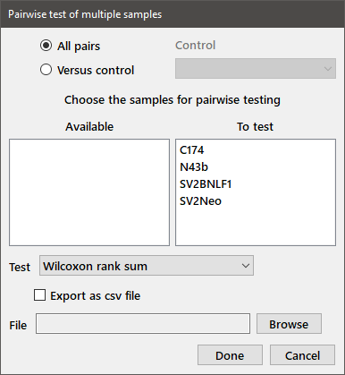
Pair-wise Wilcoxon rank sum tests, two-sided
Sample 1   Sample 2   W*       P-value     Bonf. P    FDR
SV2Neo     SV2BNLF1   -5.273   1.343e-7    8.057e-7   8.057e-7
N43b       SV2BNLF1   -4.493   7.024e-6    4.215e-5   2.107e-5
SV2Neo     C174       -3.636   0.0002765   0.001658   0.000553
N43b       C174       -3.363   0.0007718   0.004622   0.001158
C174       SV2BNLF1   -1.965   0.04941     0.2621     0.05929
SV2Neo     N43b       0.2961   0.7671      0.9998     0.7671
Note that two-sided tests are performed for the relevant pairs and the results are ordered by increasing P-value. The last two columns in the output provide the Bonferroni (Dunn-Šidák) corrected P-value and the false discovery rate.
Multiple experiments: Perform a joint analysis of replicate experiments, each consisting of two samples, x and y. The x,y pairs are selected in a Paired-sample dialog. An exact test is done if there are no ties within experiments and the product across the experiments of N!/ nx!(N-nx)! is less than 1.6×1028 (where nx is the number of x observations and N is the total number of observations in the experiment). Otherwise, Lehman's approximate test is used.
Mantel-Haenszel: A set of replicate 2 × 2 tables is chosen from the Multi-sample dialog box and tested jointly for a difference in proportions.
Combine P: Fisher's method for combining the results of statistical tests is applied to the set of P-values entered into the dialog box.

The P-values should be separated by spaces or carriage returns. The above dialog gives the output
Fisher's method for combining P-values
P-values: 0.015 0.095 0.068
X2 = 18.48 (6 df)  P = 0.005131
Adjusted P-values: The Pairwise test discussed above provides adjusted P-values and false discovery rates when multiple samples are compared using the Wilcoxon rank sum test or the Kendall or Spearman correlation tests. You may also need to adjust P-values for multiple comparisons using other statistical tests or when the P-values are obtained using other software (e.g., microarray analysis). For the example in the dialog box below, results of a microarray analysis were imported into Mstat. We chose as Source, existing variables and selected "ID_Gene" as the Labels and "P_value" as the corresponding unadjusted P-values. Since only the top 50 values are printed to the Mstat window, we selected Export as csv and provided a file name.
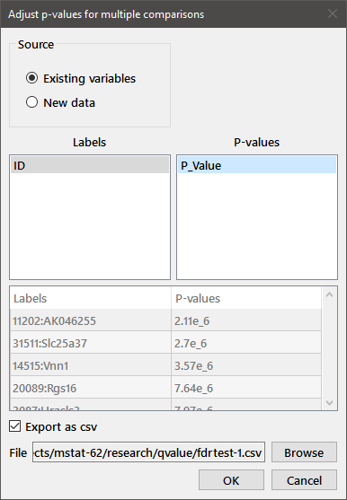
The first few lines of output to the Mstat window are:
Adjustment of p-values for multiple comparisons
Labels: ID_Gene; P-values: P_Value
Top 50 corrected p-values
Comparison                 p          Bonf. p     fdr
41373_Egfr                 5.34e-19   2.325e-14   2.325e-14
1314_Egfr                  6.21e-19   2.703e-14   1.352e-14
17543_Egfr                 8.46e-19   3.683e-14   1.228e-14
27119_1100001G20Rik        9.03e-19   3.931e-14   9.827e-15
...
Both the output table and the saved csv file list the results in order of increasing, unadjusted P-value.
You can also enter labels and unadjusted P-values into the dialog by choosing New data as the Source and filling in the table at the bottom of the dialog.
Design menu
Distributions: For the Normal distribution, the upper or lower tail probability or the value for the cumulative distribution is output for one or more z-values entered into the dialog box. For tail probabilities, the log P box may be checked and the log of the probabilities will be output. This feature is useful in the case of extreme z-values (magnitude greater than 37, which corresponds to probabilities ~10-300). Because of limitations to the precision of the algorithm used to compute Normal probabilities, the probability reported for such extreme z-values is 0. If the log P box is checked, the log of the upper bound for the probability will be given.
For the Chi-square distribution, enter the number of degrees of freedom in the upper edit box and the X2 values in the lower edit box to output the upper tail probabilities.
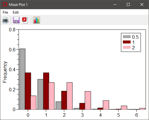
For the Poisson, binomial, hypergeometric, or negative binomial distributions, the parameters of the distribution are entered into a dialog box, as shown below for the Poisson distribution. Note that three values of the Poisson parameter, m, are entered into the edit window.

The distribution(s) from 0 to a specified value, n, in terms of the frequencies, cumulative distribution function, and/or 1-CDF, can be output for one or more distributions with the specified parameters. Alternatively, a list of frequencies for particular values of x can be output if the Specific values radiobutton is checked and the values entered in the edit box below. The above dialog box yields the output:
Poisson distribution
m = 0.5 1 2
x    f(x)                         F(x)
0     0.6065    0.3679  0.1353   0.6065 0.3679 0.1353
1     0.3033    0.3679  0.2707   0.9098 0.7358  0.406
2    0.07582    0.1839  0.2707   0.9856 0.9197 0.6767
3    0.01264   0.06131  0.1804   0.9982  0.981 0.8571
4    0.00158   0.01533 0.09022   0.9998 0.9963 0.9473
5   0.000158  0.003066 0.03609        1 0.9994 0.9834
6   1.316e-5 0.0005109 0.01203        1 0.9999 0.9955
Two parameters, m and k, are required for the negative binomial distribution, which has the form

In this form, k may take non-integer values. An alternative form of this distribution, defined as the distribution of the number of Bernoulli trials, N, required to obtain k successes when the success probability is p, for values of s=N-k is

In this case, the mean of the distribution (m) is rq/p, and k must be an integer.
Three parameters, N, p, and k, are required for the hypergeometric distribution. The distribution function is

A form familiar from analysis of 2 × 2 tables is

Sample size: The sample size required for specified values of alpha (desired P-value) and power can be estimated for measurement variables (which would be compared by the Wilcoxon rank sum test) or proportions (for which Fisher's exact test would be used). Sample sizes for case-control studies, analyzed using McNemar's test, can also be estimated.
Parameters for the Wilcoxon rank sum test are entered into the dialog box below:
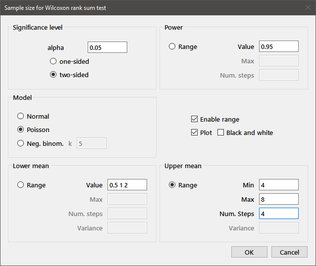
The desired value of alpha, the nature of the alternative (one- or two-sided) and the power are entered in the upper part of the panel. Three alternative data models can be chosen by radiobuttons: Normal data, for which the means and variances for both groups are entered; Poisson data, which require means for the two groups; and Negative binomial data, requiring group means and a common exponent (entered in the k edit box). The latter model is useful when studying a Poisson process where the value of the Poisson parameter is itself variable. One example of this approach applied to tumor multiplicity data can be found in Drinkwater and Klotz, Cancer Research 41:113-119, 1981.
Multiple values may be entered for Power, Lower mean, or Upper mean. Only one of these three edit boxes may have multiple values, and a single value must be entered for the three edit boxes (Min, Max, Num. steps) for the parameter that has Range enabled. Filling in the values as in the above paragraph will output the necessary sample size(s) for that collection of parameters. In order to compute sample sizes for an interval of values in one of the parameters, check the Enable range box and select one of the three radiobuttons labeled Range. Edit boxes for a maximum value and number of steps in that parameter will be enabled and you can optionally plot the result. For the above dialog box, the output is
Sample size for Wilcoxon rank sum test.
alpha=0.05 (two-sided); Power=0.95
Poisson data, Mean(lower)=0.5 1 2
Upper Mean   N/group
4            10 13 25
5            10 11 16
6            9 10 12
7            9 9 11
8            9 9 10
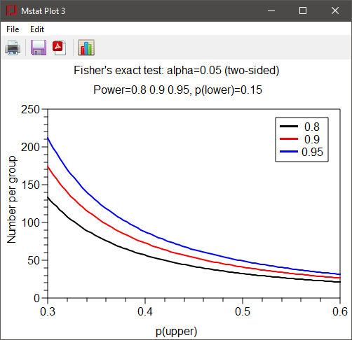
Sample sizes for Fisher's exact test are estimated for parameters entered in a dialog box similar to the one shown above. As above, multiple values may be entered for the Power, Lower proportion, or Higher proportion.
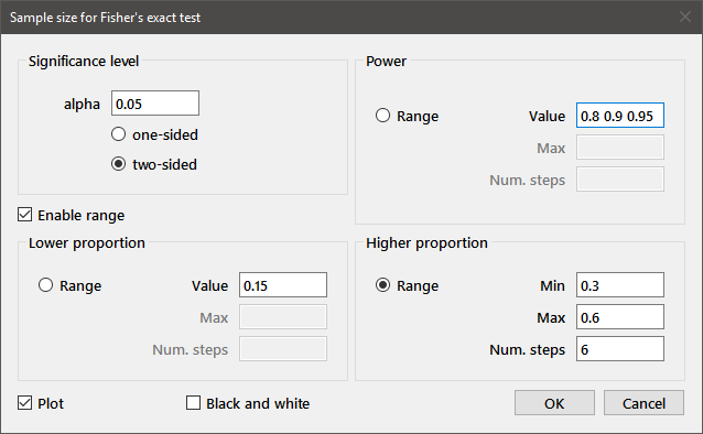
The plot generated for this set of parameters is shown below:
Sample sizes for McNemar's test are estimated by the method of Dupont (Biometrics, 44: 1157-1168, 1988). Values for alpha, the one- or two-sided alternative, and the power are entered into the dialog box as above. In addition to values for the probability of exposure in the control group (Control Proportion) and the odds ratio, the number of controls matched to each case and the correlation between cases and controls are entered in the remaining edit boxes. Sample output is shown below:
Sample size for McNemar's test.
Alpha(two-sided) = 0.05, Power = 0.9
P(control) = 0.2, Matched controls = 1, Correlation = 0
Odds ratio   Num. cases
2            226
3            83
4            50
5            36
6            29
7            25
8            22
9            19
10           18
Bayesian predictive value: Makers of diagnostic and screening tests for the presence of a particular disease focus on maximizing the sensitivity of the test, i.e., the probability that the test will yield a positive result for individuals suffering from the disease, and its specificity, the probability that a healthy individual will test negative. Bayes' theorem may be used to compute two probabilities that will be of greater interest to people who are tested. The Positive Predictive Value (PPV) is the probability that an individual who tests positive suffers from the disease. The Negative Predictive Value (NPV) is the probability that an individual who tests negative does not suffer from the disease.
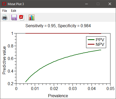
Choose Bayesian predictive value from the Design menu to compute the positive predictive value (PPV) and negative predictive value (NPV) for a diagnostic or screening test as a function of the prevalence of the disease and the sensitivity and specificty of the test. As an example, the sensitivity of an RT-PCR test for the presence of the coronavirus SARS-CoV-2 in a nasal swab sample is approximately 95% and the test's specificity is 98.4%. Enter the values in the dialog below to compute the PPV and NPV when the prevalence of infection is between 0.05% and 4.5%.

Press the OK button to close the dialog and obtain the results.
Bayesian modeling
PPV, Positive Predictive Value; NPV, Negative Predictive Value
Sensitivity = 0.95; Specificity = 0.984
Prevalence   PPV      NPV
0.005        0.2298   0.9997
0.015        0.4748   0.9992
0.025        0.6036   0.9987
0.035        0.6829   0.9982
0.045        0.7367   0.9976
The resulting plot is shown below.
Help menu
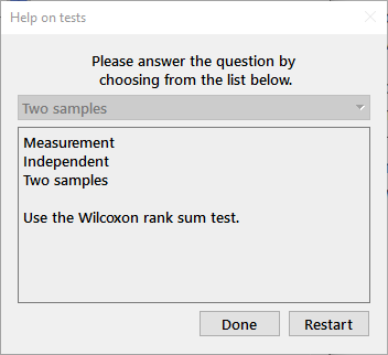
Which test?: An interactive dialog that provides help in deciding on the appropriate statistical test. Use the drop-down box to choose the answer to each question in turn and the edit window will be filled with your choices and the recommended test as shown below.
Dialog help: This menu choice toggles the dialog box help function. When activated, a window with help specific to the dialog box will be placed at the upper right of the screen. Pressing F1 or selecting this menu item will activate or inactivate the help function. Dialog help can also be activated within any dialog box by pressing Ctrl-h (Ctrl-l on macOS). An example (for McNemar's test) is shown below.
|
|
Help on Mstat: Brings up the help file for Mstat in your browser. The F1 key will also open the help file.
Check for updates: Manually check for an updated version of Mstat. Version numbers for Mstat now have the form x.y.z. Changes in x.y reflect a substantial change to Mstat. Changes at the z level generally include only minor bug fixes. If a new version of Mstat is available, you will be directed to download it from the Mstat website.
About: Shows a dialog with information on the program (see below). In particular, the version number and release date in this window, together with the operating system type and version, should be provided in any bug reports. Press the button on the left to check the Mstat website for updated software. The About menu item is in the Mstat menu on macOS.

Plug-ins menu
The Plug-ins menu provides a means to extend the capabilities of Mstat by loading J scripts that allow, for example, parsing of complex data sets or the addition of new statistical tests. A sample plug-in that generates random numbers is included in the plug-in directory. All plug-ins in that directory at the start of Mstat are loaded and displayed in the menu.
Load script: Loads any valid J script into the current Mstat session. Such scripts may define useful functions that can be accessed in the terminal window or fully fledged plug-ins. In the latter case, a menu entry is added to the end of the Plug-ins menu. Note that plug-ins loaded in this way are only available for the current Mstat session. To make the available for subsequent sessions, copy the plug-in script to the plug-in directory.
Plot window menus
The plot window contains two menus, File and Edit. Within the File menu, choosing Save will save the plot in a format (with file extension .ijg) that can be opened in a later Mstat session. To save the plot as a PDF or EPS file, choose Save as from the file menu. The resulting files may then be edited using Adobe Illustrator, the open source Inkscape drawing program, or other software. To print your plots, choose Print from the File menu. A temporary PDF file will be saved and opened in your default PDF viewer program. You can then print the plot from that program. That approach was chosen, rather than printing directly from the plot window to insure that the printed plots look identical on all platforms. Note that for PDF and EPS versions of the files, including the temporary file generated for printing, all fonts in the plot window are replaced with Helvetica. The reason for this limitation is that the font metrics for Helvetica are embedded in the program and used to generate the PDF and EPS files.
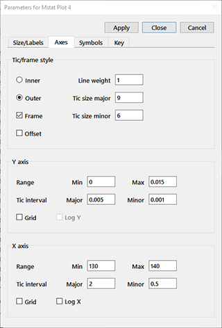
The Edit menu contains one choice, Modify plot. The Modify plot choice will bring up a tabbed dialog allowing you to change many features of the plot. Examples for each of the four tabs are shown below.
The contents of the tabs will vary depending on the type of plot.
Size/Labels: The width and height of the plot area are set in the Plot size portion of the panel. The larger edit fields in this tab allow you to modify the text shown for the plot title and X and Y axis captions. For bar graphs and dot plots, an additional field (Group names) is shown for the X axis labels; quote any entries with embedded spaces. The font sizes for each type of label may be entered in the smaller, Size edit boxes.
Axes: The Tic/frame style radiobuttons determine whether the tics are shown inside or outside of the plot frame. The weight of the frame, axes, and tics is given in the Line weight edit box, and the lengths of the major and minor tics in Tic size major and Tic size minor, respectively. Checking the Frame box places a frame around the plot; checking the Offset box will move the axis origins slightly away from the lower left corner of the frame. For each axis, you can enter the minimum and maximum for the range and the major and minor tic intervals in the indicated edit boxes. The two check boxes specify whether a grid (faint lines at the major tic intervals) or log axis is shown. The Log check box is disabled if any of the values are less than or equal to zero. Only the Y axis is shown for dot plots or any of the bar graph types.

|
|
|
|
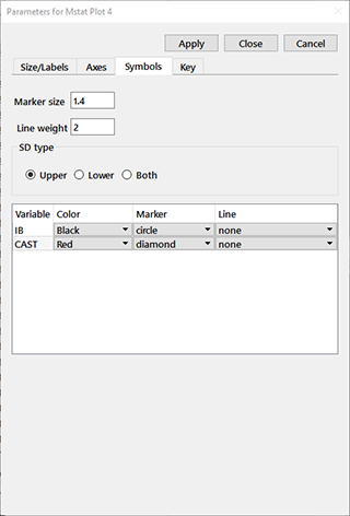
Symbols: An edit box for Line weight is shown for any of the XY plots, Kaplan-Meier plots, power plots, or regression analyses. A Marker size edit box is available for the XY plot types, regression plots, and dot plots. The Marker with SD plot type will also have a set of radiobuttons allowing you to specify whether the vertical bar indicating the standard deviation is shown above, below, or above and below the marker. The remainder of the tab consists of a table with an entry for each plotted variable. For each variable, you may set the color for the markers, lines, or bars from the 22 entries in the dropdown listbox. For plots with markers, choose from among circle, diamond, square, triangle, plus, times, vbar (vertical bar), opencircle, opendiamond, opensquare, opentriangle, or none. Choices for plots with lines include none, solid, dash, dot, '-.' (dash-dot), and '-..' (dash-dot-dot). If you plan to edit your graph in Adobe Illustrator, select solid lines using colors to differentiate among the lines in the plot and apply the desired line style in Illustrator. The dashed and other broken line styles are saved as individual elements in PDF or EPS files.
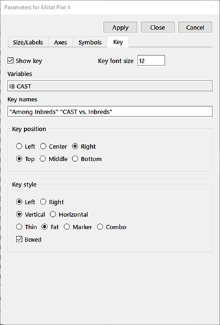
Key: The Show key check box determines whether a key is displayed on the plot. Note that keys are disabled for both dot plots and regression plots. The Key font size edit box contains the font size for the text. The variables, in the order shown in the key, are displayed in the Variables edit box. You can specify the text to be shown for each in Key names; values with embedded spaces must be quoted. The location of the key is determined by the two sets of radiobuttons in the Key position group. As of this writing, the Center choice displays at the left of the plot. The Key style group controls various aspects of the appearance of the key, including whether the marker/color block appears to the left or right of the text, whether the key is arranged vertically or horizontally, the appearance of the marker/color block, and whether a box is placed around the key.