Tutorial
This tutorial will work through a short Mstat session to familiarize you with the operation of the program. A more comprehensive reference section follows.
In the examples below, you have tumor multiplicity data for two groups of animals (heterozygous or homozygous for a particular locus) and want to test the hypothesis that the genotypes differ in their cancer risk. The data are:
| homozygous | 0 0 0 4 6 7 20 1 19 14 8 19 5 16 26 3 2 16 1 2 1 0 12 12 1 0 0 0 0 6 5 0 5 0 0 5 1 0 2 0 11 6 0 3 0 6 0 |
| heterozygous | 5 10 28 5 27 0 19 10 26 1 53 2 49 38 21 15 25 18 1 71 1 15 18 3 44 2 3 74 52 37 7 12 26 58 9 2 2 12 35 0 18 2 1 0 3 6 3 6 28 2 |
We will also import similar data from an Excel spreadsheet that was saved as a "CSV" (comma-separated variable) file.
Starting the program.
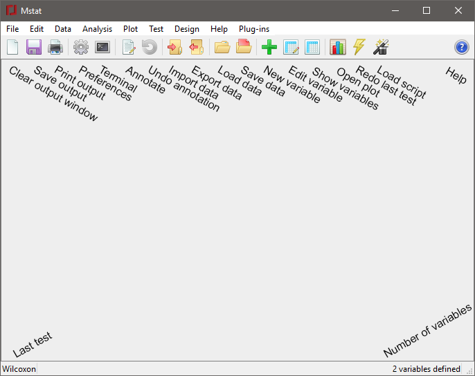
Start the program by clicking on the Mstat entry in Start Programs (Win), double-clicking the Mstat icon in the Mstat 8.1 folder (Mac), or entering mstat81/mstat from the terminal (Linux). The main program window (see below) consists of a menu bar and toolbar for choosing program functions, an output window for displaying your results, and a statusbar that displays information about the current session. Each toolbar button is equivalent to a menu entry, except for the Redo last test button, which is assigned to the most recently chosen item from the Analysis, Test, or Design menus. Although it's not shown in the screenshot, when the program starts (or the output window is cleared), the version number and current date and time are printed as the first line of the output window.
Entering and editing data.
The three data types in Mstat are stored as arrays (lists) of numbers or character strings or as tables (Variables, Indicators, and Tables, respectively). An Indicator stores a list of non-numeric values that can be used to subdivide a regular variable into various groups (see example below). It could also be used to store a list of labels for a bar graph.
The name for an Mstat variable can be of any length, must start with a letter, and consists of a sequence of letters, numeric digits, or the underscore character (no spaces, punctuation marks, or other special characters; the name cannot contain a double underscore or end in an underscore). Variable names are case-sensitive, i.e., "Mutant", "mutant", and "MuTaNt" all refer to distinct variables. The same name can be used simultaneously for each of the three data types (at the cost of some confusion), but within each type, every variable name must be unique. You should try to choose variable names that are meaningful to you. Mstat variables may be stored on disk as text files (see below) so all of the data entered in an Mstat session may be reloaded into the program for later use.
In order to define a new variable, choose New from the Data menu, or click on the New variable button on the toolbar. You will then see the following dialog box:
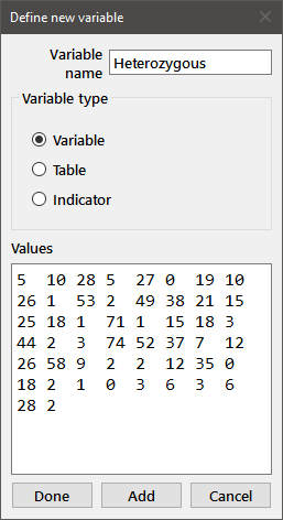
Enter your new variable name (in this case Heterozygous) in the upper window, select the appropriate variable type from among the radiobuttons, and tab to the larger window to enter your data. You should enter numbers in simple (e.g., 1 3.5 2.0215) or exponential (e.g., 3.2e-5) format separated by spaces or carriage-returns. When you have finished entering the data, click on the Add button (if you wish to define additional variables) or the Done button.
Several features will make it easier to enter data into Mstat. First, you can use J notation to define the data (see Reference section). You will most often use this feature for entering repeated values. For example, the six values of "2" could be specified as (6#2) [the parentheses aren't required but are advisable]. You can also paste data from the clipboard into the large edit window. For example, if your data were in an Excel file, you could open the spreadsheet, highlight the column or row of cells that contained the desired data, copy it to the clipboard, and paste it into the edit window (tabs or other white space characters are ignored). Other ways of bringing data into the program include loading a saved Mstat data file and importing tab or comma-delimited text files.
Mstat does some simple error checking to help with data entry. For a regular variable, if the edit window contains non-numeric data (or data that doesn't evaluate to a list of numbers in J), you will see an error message, and you'll be given the opportunity to edit the data. If you chose a variable name that is already defined, you will also get an error message and the chance to enter a new name. After Adding the data, the dialog box will be cleared, and you can define an additional variable. Do that to define the Homozygous variable. Try copying the data from this help file and pasting it into the edit window.
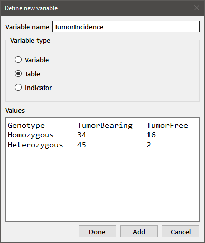
Both the Heterozygous and Homozygous variables are simple one-dimensional data arrays. You can also enter data in a tabular form that is appropriate for contingency tables. Define a new variable and select the Table radiobutton. You can enter the data as a table in the edit box with appropriate column and row headings. Entry is free form (i.e., the number of spaces separating the entries doesn't matter), but you must have a line with the column headings, followed by one line for each row in the table. The column and row headings must each be one word consisting of alphanumeric characters (with no spaces within the name). The label for the column of row labels ("Genotype" in this case) is optional. Note that you can resize the dialog box for convenience.
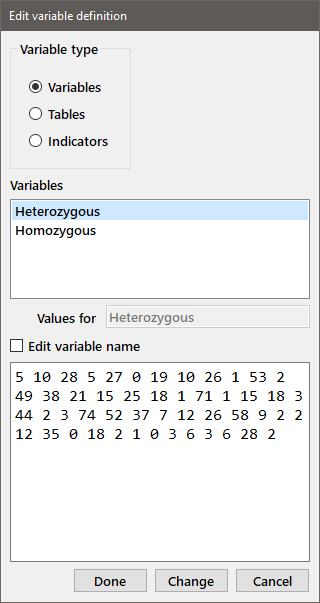
If you find that you have entered some of the data incorrectly (e.g., after you've used the Show function to print the data to the output window), you can edit the variable by choosing Edit from the Data menu or by clicking the Edit data button on the toolbar. You will get the following dialog box below.
Select the appropriate variable type, choose the name of the variable to be edited from the list box (highlight the desired name and double-click or press enter). The data associated with that variable will be displayed for editing in the window below. If you want to change the name of the variable, select the Edit variable name checkbox to enable the variable name edit box. When you have finished modifying the data (or variable name), press the Change or Done button. The dialog box will stay open to allow additional editing until Done is pressed.
Show the data in the output window.
In order to make sure that you've correctly entered the data, print the variables to the output window by choosing Show from the Data menu or pressing the Show data button on the toolbar. Select the desired variable type, select (highlight and double-click or press Enter) the variable(s) you want to show from the Available variables list and its name will move from the list box on the left to that on the right of the window. You can also highlight multiple variables and move them from one list to the other by dragging and dropping. Dragging and dropping within one of the lists will reorder the variables. When you have selected all of the variables and put them in the desired order, press Done to show the contents of the variables. If you want to print the contents of another variable type to the output window, you will need to reopen the dialog box.
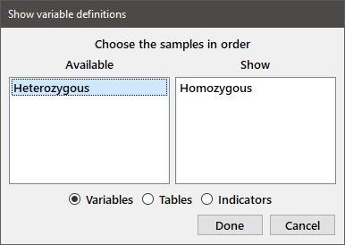
After choosing the two available variables and then reopening the dialog box to choose the table, you should see the following in the output window:
Homozygous
0  0  0  4  6  7  20 1  19 14 8  19 5  16 26 3
2  16 1  2  1  0  12 12 1  0  0  0  0  6  5  0
5  0  0  5  1  0  2  0  11 6  0  3  0  6  0

Heterozygous
5  10 28 5  27 0  19 10 26 1  53 2  49 38 21 15
25 18 1  71 1  15 18 3  44 2  3  74 52 37 7  12
26 58 9  2  2  12 35 0  18 2  1  0  3  6  3  6
28 2

Table TumorIncidence
Genotype      TumorBearing  TumorFree
Homozygous    34            16
Heterozygous  45            3
Importing data.
You can import data into an Mstat session from a tab-delimited or comma-delimited text file, such as those produced by spreadsheet programs like Microsoft Excel or LibreOffice Calc. Choose Import data from the File menu and select the file, tutorial.csv, from the file open dialog and you will get a dialog box as follows:
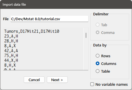
The file name appears in the edit box at the top of the dialog and the first lines of the file appear in the edit window below it. Based on the contents of the file, the appropriate radiobutton for the delimiter (comma in this case) is selected. The set of radiobuttons in the Data by group allow you to specify whether the data in the file should be read by rows or columns, or the table should be imported as a whole as a table variable (see below). If the first row (for column format), or first column (for row format) does not contain the names of the variables, check the No var. names box and you will be prompted for variable names. When you've made the appropriate choices, press the Next button to bring up the following dialog (in the case that you've chosen to import the data by rows or columns):
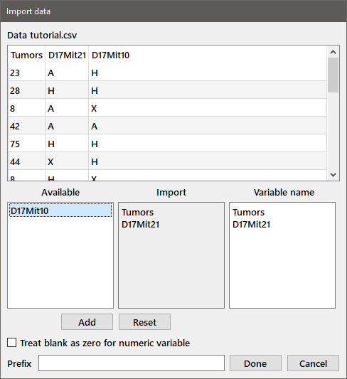
The parsed data are shown in the table at the top of the dialog. Note that the first column contains numeric data, but the second two contain non-numeric data. These latter two columns would be converted to indicator variables (see below) while the former would be saved as a regular variable. The available variables are listed in the listbox at the bottom left. You can choose to import any or all of them by double-clicking the column name(s) or selecting one or more names and pressing Add. The names of the columns to be imported will be moved over to the Import box, with the variable name to be used displayed in the third edit box, which can be modified if desired. If you are importing multiple data sets, you can automatically prefix the variable names with the value in the Prefix box. For example, if you entered "X201" in the Prefix box, the variable name for "Tumors" would become "X201_Tumors". If a column (or row) of numeric data contains blank cells, the blank cells are ignored by default. If you want the blank cells to be recorded as "0" values, check the box labeled "Treat blank as zero". Press Done to import the variables.
If you want to import the table as a whole, choose the Table radiobutton from the Data by group. If all of the data in a column, except the first entry, are numeric, the data in the column will be converted to numbers unless you check the No numeric conv. box.
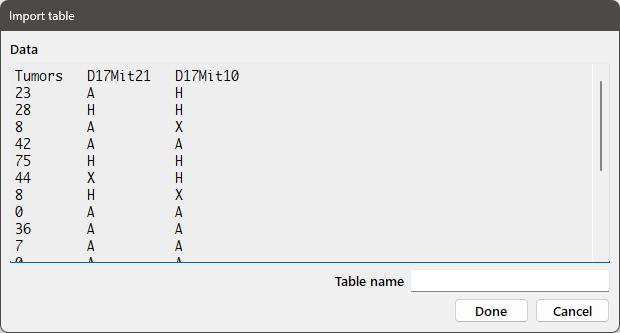
Pressing Next will bring up the following dialog box:

Enter the desired variable name for the table in the Table name edit box and press Done to import the table.
Indicator variables.
Indicator variables allow you to partition a regular variable (or another indicator variable) into subgroups based on the value of the indicator variable. Both variables must have the same number of values. In our example above, we imported a set of numeric observations (Tumors) and a single indicator variable (D17Mit21), which contains the genotype at a particular locus for each observation represented in the Tumors variable. Although, in this case, each indicator is represented by a single character (A, H, or X), an indicator variable can contain any arbitrary data (for example, the entries could be "homozygous", "heterozygous", and "unknown"). Leading and trailing spaces in the data are removed during the import.
To subdivide a regular variable according to an indicator, choose Classify from the Data menu to get the following dialog box:
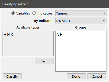
The radiobuttons allow you to select indicator or regular variables as the target for classification (variables in this case). The variable "Tumors" is chosen in the top dropbox and the desired indicator variable, "D17Mit21", is chosen from the one immediately below. The distinct entries contained in the indicator variable are shown in the edit box at the left of the dialog. Enter the types that you wish to use to partition the variable in the Groups edit box exactly as they appear in the Available types box. Press the Each button if you want to partition the variable by all of the available types. Pressing the Classify or Done button in our example will generate two new variables, with names of the form Variable_Indicator_Type. The Classify button will keep the dialog box open so that additional variables can be partitioned. In our case, we will make two new variables, Tumors_D17Mit21_A and Tumors_D17Mit21_H, that divide the Tumors variable into two groups, those observations for which the associated type is A and those of type H. Showing the new variables to the output window gives
Tumors_D17Mit21_A
23 8  42 0  36 7  0  5  2  8  16 5  5  13 3  7
4  5  4  3  4  5  3  2  2  25 5  0  3  11 29

Tumors_D17Mit21_H
28 75 8  16 45 44 69 57 47 45 30 39 25 15 26 8
25 50 10 44 0  12 47 29
Describing data.
The analysis menu has several choices useful for describing your data, including tabulating the means, variances, and quantiles for several variables, or the sample distributions for one or more variables, as well as some simple data plots.
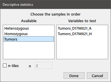
To display the means and standard deviations of some of your variables, choose Descriptive from the Analysis menu to obtain the following dialog box.
Choose the desired variables in the order that you want them to appear in the output table by double-clicking the name in the Available variables list or highlighting the name and pressing Enter. You can also move variable names between the Available and Variables to test boxes by dragging and dropping. If you check the n-tiles box and enter 4 in the box immediately below it, the output table will also display the data values for the 1st, 2nd, and 3rd quartiles, as well as the minimum and maximum observations. (To show only the median, enter "2" in the box labeled n.) Press Done to display the output.
Descriptive statistics
Sample             N   Mean    Std. dev.  4-tile        Min  Max
Tumors_D17Mit21_A  31  9.194   10.73      3 5 9.5       0    42
Tumors_D17Mit21_H  24  33.08   19.82      15.5 29.5 46  0    75
Graphical plots of your data can often provide helpful insights and are obviously useful for explaining your results to other people. Mstat does a number of fairly simple plots, including histograms of sample distributions, a variety of bar graphs, survival plots, X-Y plots for bivariate data, regression curves, power plots, and dot plots for comparing several sample distributions.
Choose Dot plot from the Plot menu and select both variables as described above for Descriptive statistics to get the following dialog box:
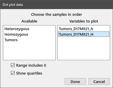
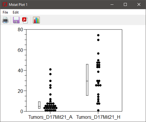
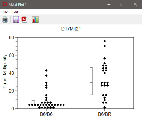
If you want your plot to have an origin of 0 on the Y-axis, check the Range includes 0 box. To display a bar indicating the median and first and third quartiles next to the data points, select the Show quartiles box. Note that the bar may partially obscure some of the data points. Press Done and you will see the window below.
The menu choices or four buttons at the top of the window will allow you to print, save, save as pdf or eps, and change the properties of the plot, respectively. The plot will be printed or saved in the same shape and approximately the same size as it is shown on screen. Plots may also be saved as PDF or EPS files, which may be printed or edited in Adobe Illustrator, Affinity Designer, the open source Inkscape drawing program, or other applications.
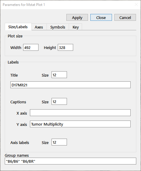
Press the Modify plot button (the rightmost button) to get the dialog below. The four tabs allow you to modify the size of the plot, the size or text of the labels or captions; the ranges of the axes, tic size or tic interval; the shape, size, or color of the symbols; and the contents or position of the plot key. For our plot, change the Group names on the X axis to "B6/B6" and "B6/BR", enter the text "D17Mit21" in the title box, and add a Y-axis label (Tumor multiplicity). Change to the Symbols tab and use the dropdown box to change the Marker to a diamond. After making the modifications indicated above, press Apply (to leave the Modify plot dialog open) or Close and the plot will be redrawn.
You can have multiple plots open at the same time. If you don't close the plot window (by clicking the close button at the upper right border), all open plots will be closed when you exit the program. Choose File > Print or press the Print button and the plot will open in your default PDF viewer (e.g., Acrobat reader). The plot can then be printed from that application. To save your plot for later modification, select File > Save or press the Save button. As noted above, you may also save your plot as a PDF or EPS file by choosing File > Save as or pressing the Save as button.
Statistical tests.
The appropriate test depends on the number of samples (two-sample and multisample tests), whether the data are categorical (observations that fall in a set of mutually exclusive categories) or measurements (e.g., number of colonies, phosphorimager counts, etc.), and whether you are testing against an ordered alternative (one-sided) or a more general alternative hypothesis (two-sided). Most of the tests implemented in Mstat are summarized in the table below (the links will take you to the appropriate section of the Notes for descriptions of the tests). Two tests not included in the table are the one-sample Goodness of Fit test and the Mantel-Haenszel test, which allows the joint analysis of multiple 2 × 2 tables. You can get interactive help on choosing the right test by selecting Which test? from the Help menu.
| Statistical question | Alternative hypothesis |
Two samples | Multiple samples |
| Difference in location, independent measurements | ordered | Wilcoxon rank sum | Jonckheere-Terpstra |
| general | Wilcoxon rank sum | Kruskal-Wallis | |
| Difference in location, paired measurements |
ordered or general |
Wilcoxon signed rank |
|
| Difference in dispersion, independent measurements | ordered | Miller jackknife | |
| general | Miller jackknife | Conover | |
| Difference in proportions, binary classification, independent samples | ordered |
Fisher’s exact or Barnard’s exact |
Cochran-Armitage |
| general |
Fisher’s exact, Barnard’s exact or Chi-square |
Chi-square | |
| Difference in proportions, binary classification, paired samples |
ordered or general |
McNemar |
|
| Difference in proportions, multiple categories | general | Chi-square or Likelihood ratio | Chi-square or Likelihood ratio |
| Difference in survival (with censored data) | general | Logrank | Logrank |
| Correlation |
ordered or general |
Kendall’s or Spearman’s rank correlation test |
|
| Parallelism of two or more lines |
ordered or general |
Sen-Adichie | Sen-Adichie |
In order to perform a two-sample test (e.g., Wilcoxon rank sum, Wilcoxon signed rank, Kendall's rank correlation), choose the appropriate test from the Test menu and you will see a dialog box similar to that shown below. For our data, choose Wilcoxon from the Test menu.
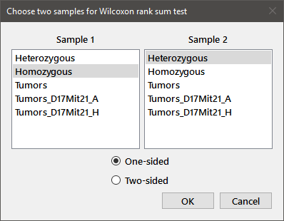
The name of the test is shown in the title bar, and the two listboxes will contain all of the currently defined regular variables. Choose one variable from each listbox, check the appropriate radiobutton for a one-sided or two-sided test, and press OK. The results of the test will appear in the output window.
Wilcoxon rank sum test
Sample         N    Mean    St. dev.
Homozygous     47   5.213   6.669
Heterozygous   50   18.1    19.53
W = 1745.5   W* = -4.132
Approx, P(one-sided) = 1.795e-5
One-sided alternative: Homozygous < Heterozygous
The output shows a table with the number of observations, mean, and standard deviation for the two samples. The table is followed by the rank sum statistic and the normalized form of the statistic. The second last line provides the P-value. When no ties are present and the total number of observations is less than 200, an exact P-value is computed for the rank sum statistic. If ties are present and the total number of observations is less than or equal to 20, an exact test is performed (labeled CondExact) but the P-value is conditional on the pattern of ties. Despite this conditional nature, the performance of the test is still better than the approximate test. In all other cases, an approximate P-value (labeled Approx) is shown. This value is based on an Edgeworth approximation due to Hodges et al., and is corrected for ties and continuity (see the Notes for further details). The last line indicates the direction of the one-sided test that gave the P-value. If you had the other direction in mind (i.e., Homozygous > Heterozygous), the appropriate P-value is the complement (1-P) of the value printed out.
Categorical data are stored as tables, like the TumorIncidence table we entered above. Fisher's exact, Barnard's exact, and the Chi-square tests all allow analysis of a set of one or more tables. Choose Fisher's exact from the Test menu to get the following dialog box:
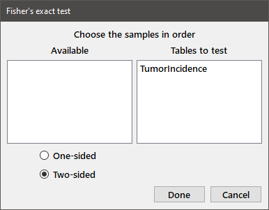
Select the desired table(s) in the Available box by double-clicking on each or highlight them and press Enter to move them to the Tables to test box. You can also drag and drop one or more table names. Choose a one- or two-sided test by selecting the appropriate radiobutton, then press Done. You should see the following in the output window:
Fisher's exact test
Table TumorIncidence
Genotype      TumorBearing  TumorFree  Total
Homozygous    34            16         50
Heterozygous  45            2          47
Total         79            18         97
P(two-sided) = 0.0004636
Saving output and data files.
When you've completed a session (or periodically during lengthy data entry sessions), you can save the current data set by choosing Save data from the File menu, or pressing the Save data button. You will get a standard File save dialog. You can print the contents of the output window to the current default printer by choosing Print from the File menu (or pressing the Print output button) and save it to a text file by choosing Save output from the File menu. When you quit the program (choose Exit from the File menu), you will be prompted to save both the data and the output window if the files are not up to date.